Labyrinth

In short, we’re given a grid with walls and free cells, and a start ($A$) and end ($B$) point. We must find the shortest path from $A$ to $B$. In the figure below, the blue cells are the walls and the green cells are the two points we want to find a path between:

At first glance, it may seem like this problem has nothing to do with what we spent the last few articles learning about. This is a grid. Where’s the graph?!

Well…

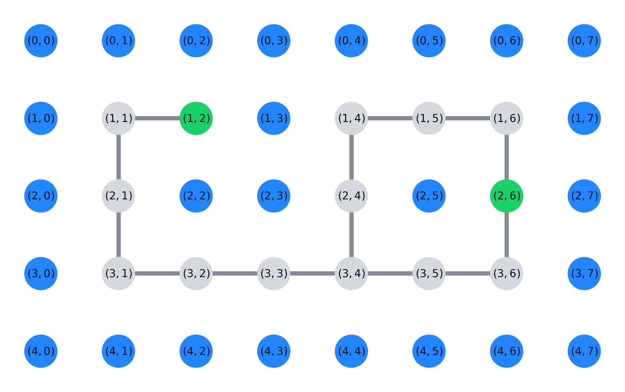
We can easily interpret any such grid as a graph by treating each cell ($(i,j)$) as a node, and then adding an edge from $(i,j)$ to $\{(i+1,j), (i-1,j), (i,j+1), (i,j-1)\}$ provided:

• The destination cell exists (no out-of-bounds)
• Both the cells we’re adding an edge to are not wall cells.

Since we want the shortest path between the two green cells, we’ll use a breadth-first search (why does BFS find the shortest path? We’ll talk more about this later!).

So far, we’ve only seen how to check whether a path between two nodes exists. We don’t really have a way to find that path.

BFS Tree

A fancy term for a relatively simple concept, a BFS tree is a tree that is formed by the following process:

• First, create an empty graph with the same nodes as the original graph, but with no edges.
• For all nodes that are not the node we begin our BFS from ($u$), keep track of the node that pushed us onto the queue ($p$).
• Add edge $p \to u$ to the tree.

Recall that one of the key properties of a tree is that there is exactly one way to get from one node to another. A key property of the BFS tree is that the one way to get from specifically the root of the tree to any other chosen node will be the shortest path to do so.

The solution now becomes clear: we run a breadth-first search from $A$ and keep track of parent nodes. Then, we start from $B$ and keep descending up the tree by going to our parent repeatedly until we reach $A$. The rest are implementation details (and the implementation for this problem is pretty involved, so you should try it yourself!)